Chapter 5 Simulation and Statistical Models
5.1 Prediction Uncertainty
This chapter will focus on how we can use simulation to improve our statistical models, provide more clarity about causal effects and begin to build upon the framework used to estimate causal effects.
Thus far, we have only discussed the point estimates of a logit/probit model. But, we also need to discuss the variances of the estimates, in order to derive standard errors and test-statistics. Typically, when we use maximum likelihood, we can use the matrix of second derivatives to calculate the variance of a parameter.
First, let’s define the Hessian as the matrix of second derivatives for our parameters. As noted by Long (1997, p.32)
\[H(\theta)={{\partial^2 ln L(\theta) }\over{\partial \theta \partial \theta^T}}\]
What does the second derivative tell us? If the first derivative is the instantaneous effect of \(x\) on \(y\). The second derivative is the rate of change. For instance, we previously used it to determine whether a function is concave (upside down u) or convex (u) shaped. If a function is concave, and we find the global maximum, the first derivative will be 0 and the second derivative will be negative. If it’s convex, it will be positive.
The negative of the expected value of the Hessian is the information matrix,
\[I(\theta)=-E(H(\theta))\].
The inverse of the information matrix is the variance-covariance matrix for the parameters.
\[V(\theta)=[-E(H(\theta))]^{-1}\].
We can display the estimated variance matrix by using the \(\texttt{vcov}\) statement.
library(dplyr)
load("~/Dropbox/github_repos/teaching/POL683_Fall24/advancedRegression/vignettes/dataActive.rda")
dat = dataActive %>% mutate( support_protest = ifelse(violent >3, 1, 0)) %>%
  select(support_protest, VIOLENT)
# Estimate logit
logitModel = glm(support_protest ~ VIOLENT, data = dat,
                 family = binomial(link = "logit"))
logitModel
##
## Call: glm(formula = support_protest ~ VIOLENT, family = binomial(link = "logit"),
## data = dat)
##
## Coefficients:
## (Intercept) VIOLENT
## -0.3419 -0.5526
##
## Degrees of Freedom: 3599 Total (i.e. Null); 3598 Residual
## Null Deviance: 4671
## Residual Deviance: 4609 AIC: 4613The variance-covariance matrix of the parameters can be used to simulate the distribution of the predicted probabilities.
##             (Intercept)      VIOLENT
## (Intercept)   0.0023083 -0.002308300
## VIOLENT      -0.0023083  0.004981626
So this is the variance-covariance matrix of parameters. We could then simulate from a multivariate normal density, where the means correspond to the regression parameter estimates – from the model – and a variance-covariance matrix of these estimates.
##             (Intercept)      VIOLENT
## (Intercept)   0.0023083 -0.002308300
## VIOLENT      -0.0023083  0.004981626
## (Intercept) VIOLENT
## [1,] -0.3050387 -0.6383429
## [2,] -0.3741993 -0.5397935
## [3,] -0.3004893 -0.5504543
## [4,] -0.2894388 -0.6500024
## [5,] -0.3556048 -0.6477099
## [6,] -0.2809330 -0.6832987
## [7,] -0.3690994 -0.4242484
## [8,] -0.3184905 -0.5689466
## [9,] -0.3558240 -0.6148524
## [10,] -0.3366557 -0.5328848- The treatment effect
library(dplyr)
library(plotly)

simval %>%
  as.data.frame() %>%
  mutate(
    y = 1 / (1 + exp(-(logitModel$coefficients["(Intercept)"] + logitModel$coefficients["VIOLENT"] * VIOLENT)))
  ) %>%
  plot_ly() %>%
  add_histogram(x = ~y, nbinsx = 100, name = "Predicted Probabilities") %>%
  layout(
    title = "Predicted Probabilities",
    xaxis = list(title = "Probability"),
    yaxis = list(title = "Frequency")
  )
5.2 Marginal Effects
It can often be useful to calculate the marginal effect of a variable – i.e., the change in probabilities for a one unit increase in the variable. Given how I’ve coded my data, a “one-unit” change corresponds to the following.
\(\Delta x_i =x_{i,1}-x_{i,0}\)
For y, the marginal value is then.
\(\Delta y=f\left(x_{i,1},\ldots,x_n \right)-f\left(x_{i,0},\ldots,x_n \right)\)
And the marginal effect is (if a unit change, then the denominator is 1):
\(\frac{\Delta y}{\Delta x}=\frac{f\left(x_{i,1},\ldots,x_n \right)-f\left(x_{i,0},\ldots,x_n \right)}{x_{i,1}-x_{i,0}}\)
So,
Calculate the probability that \(y=1\) when \(x=0\).
Calculate the probability that \(y=1\) when \(x=1\).
Subtract (1) from (2)
We might simulate a confidence interval as well, by modifying the recipe.
Calculate the probability that \(y=1\) when \(x=0\) by drawing \(K\) draws from the multivariate normal of the model, with mean values corresponding to the slopes and the variance covariance matrix of the model parameters.
Calculate the probability that \(y=1\) when \(x=1\) by drawing \(K\) draws from the multivariate normal of the model, with mean values corresponding to the slopes and the variance covariance matrix of the model parameters.
Subtract (1) from (2), which will now yield a distribution.
5.3 The Normal Distribution
The normal – Gaussian – distribution plays an important role in statistics. The reason is fairly obvious: many phenomean are normally distributed. Think of the central limit theorem, or more generally, the distribution of natural phenemona. We’ve discussed the logit regression, and the role that maximum likelihood plays in estimating model parameter, but we can actually do the identical thing with a linear model
set.seed(123)
n <- 100
x <- rnorm(n, 0, 1)
y <- 0.25 + 0.25 * x + rnorm(n, 0, 0.5)

intercept_grid <- seq(0, 1, length.out = 100)
slope_grid <- seq(0, 1, length.out = 100)
sigma <- 1  # Assume known sigma for simplicity

# initialize the likelihood matrix. We'll fill this in as we go.
# Basically we're going to calculate the likelihood for each combination of intercept and slope
likelihood <- matrix(0, nrow = length(intercept_grid), ncol = length(slope_grid))

for (i in 1:length(intercept_grid)) {
  for (j in 1:length(slope_grid)) {
    intercept <- intercept_grid[i]
    slope <- slope_grid[j]
    y_pred <- intercept + slope * x
    likelihood[i, j] <- prod(dnorm(y, mean = y_pred, sd = sigma))
  }
}

  # Plot in 3d
 dat %>% plot_ly(x = ~intercept_grid, y = ~slope_grid, z = ~likelihood) %>%
  add_surface(type = "scatter3d",  colorscale = list(c(0,1),c("lightgrey","black")))  %>%
  layout(
    scene = list(
      xaxis = list(title = 'Intercept'),
      yaxis = list(title = 'Slope'),
      zaxis = list(title = 'Likelihood'),
      scene = list(
      )
    )
    )
5.4 The Posterior Distribution
Imagine our interest is in predicting a feeling thermometer score, using a person’s ideology, \(x_i\). The feeling thermometer score ranges from 0 to 100.
Consistent with McElreath (2021), let’s write the scientific model like this:
\[ y_{feeling} \sim Normal(\mu_i, \sigma)\\ \mu_i = \beta_0 + \beta_1 (x_i - \bar{x})\\ \beta_0 \sim Normal(0, 10)\\ \beta_1 \sim Normal(0, 10)\\ \sigma \sim Uniform(0, 50) \]
We’ll sample from the posterior in a variety of ways. Let’s start using \(\texttt{stan}\)/\(\texttt{brms}\).
library(brms)

n <- 100
x <- rnorm(n, 0, 1)
y <- 2 + 3 * (x - mean(x)) + rnorm(n, 0, 1)
data <- data.frame(x = x, y = y)

# Define the model formula
formula <- bf(y ~ x - mean(x))

# Specify the priors
priors <- c(
  prior(normal(0, 10), class = "b"),
  prior(normal(0, 10), class = "Intercept"),
  prior(uniform(0, 50), class = "sigma")
)

# Fit the model
fit <- brm(formula, data = data, prior = priors, chains = 4, iter = 2000, warmup = 1000)
## Running /Library/Frameworks/R.framework/Resources/bin/R CMD SHLIB foo.c
## using C compiler: ‘Apple clang version 16.0.0 (clang-1600.0.26.4)’
## using SDK: ‘’
## clang -arch arm64 -I"/Library/Frameworks/R.framework/Resources/include" -DNDEBUG -I"/Library/Frameworks/R.framework/Versions/4.3-arm64/Resources/library/Rcpp/include/" -I"/Library/Frameworks/R.framework/Versions/4.3-arm64/Resources/library/RcppEigen/include/" -I"/Library/Frameworks/R.framework/Versions/4.3-arm64/Resources/library/RcppEigen/include/unsupported" -I"/Library/Frameworks/R.framework/Versions/4.3-arm64/Resources/library/BH/include" -I"/Library/Frameworks/R.framework/Versions/4.3-arm64/Resources/library/StanHeaders/include/src/" -I"/Library/Frameworks/R.framework/Versions/4.3-arm64/Resources/library/StanHeaders/include/" -I"/Library/Frameworks/R.framework/Versions/4.3-arm64/Resources/library/RcppParallel/include/" -I"/Library/Frameworks/R.framework/Versions/4.3-arm64/Resources/library/rstan/include" -DEIGEN_NO_DEBUG -DBOOST_DISABLE_ASSERTS -DBOOST_PENDING_INTEGER_LOG2_HPP -DSTAN_THREADS -DUSE_STANC3 -DSTRICT_R_HEADERS -DBOOST_PHOENIX_NO_VARIADIC_EXPRESSION -D_HAS_AUTO_PTR_ETC=0 -include '/Library/Frameworks/R.framework/Versions/4.3-arm64/Resources/library/StanHeaders/include/stan/math/prim/fun/Eigen.hpp' -D_REENTRANT -DRCPP_PARALLEL_USE_TBB=1 -I/opt/R/arm64/include -fPIC -falign-functions=64 -Wall -g -O2 -c foo.c -o foo.o
## In file included from <built-in>:1:
## In file included from /Library/Frameworks/R.framework/Versions/4.3-arm64/Resources/library/StanHeaders/include/stan/math/prim/fun/Eigen.hpp:22:
## In file included from /Library/Frameworks/R.framework/Versions/4.3-arm64/Resources/library/RcppEigen/include/Eigen/Dense:1:
## In file included from /Library/Frameworks/R.framework/Versions/4.3-arm64/Resources/library/RcppEigen/include/Eigen/Core:19:
## /Library/Frameworks/R.framework/Versions/4.3-arm64/Resources/library/RcppEigen/include/Eigen/src/Core/util/Macros.h:679:10: fatal error: 'cmath' file not found
## 679 | #include <cmath>
## | ^~~~~~~
## 1 error generated.
## make: *** [foo.o] Error 1
##
## SAMPLING FOR MODEL 'anon_model' NOW (CHAIN 1).
## Chain 1:
## Chain 1: Gradient evaluation took 2.6e-05 seconds
## Chain 1: 1000 transitions using 10 leapfrog steps per transition would take 0.26 seconds.
## Chain 1: Adjust your expectations accordingly!
## Chain 1:
## Chain 1:
## Chain 1: Iteration: 1 / 2000 [ 0%] (Warmup)
## Chain 1: Iteration: 200 / 2000 [ 10%] (Warmup)
## Chain 1: Iteration: 400 / 2000 [ 20%] (Warmup)
## Chain 1: Iteration: 600 / 2000 [ 30%] (Warmup)
## Chain 1: Iteration: 800 / 2000 [ 40%] (Warmup)
## Chain 1: Iteration: 1000 / 2000 [ 50%] (Warmup)
## Chain 1: Iteration: 1001 / 2000 [ 50%] (Sampling)
## Chain 1: Iteration: 1200 / 2000 [ 60%] (Sampling)
## Chain 1: Iteration: 1400 / 2000 [ 70%] (Sampling)
## Chain 1: Iteration: 1600 / 2000 [ 80%] (Sampling)
## Chain 1: Iteration: 1800 / 2000 [ 90%] (Sampling)
## Chain 1: Iteration: 2000 / 2000 [100%] (Sampling)
## Chain 1:
## Chain 1: Elapsed Time: 0.011 seconds (Warm-up)
## Chain 1: 0.008 seconds (Sampling)
## Chain 1: 0.019 seconds (Total)
## Chain 1:
##
## SAMPLING FOR MODEL 'anon_model' NOW (CHAIN 2).
## Chain 2:
## Chain 2: Gradient evaluation took 4e-06 seconds
## Chain 2: 1000 transitions using 10 leapfrog steps per transition would take 0.04 seconds.
## Chain 2: Adjust your expectations accordingly!
## Chain 2:
## Chain 2:
## Chain 2: Iteration: 1 / 2000 [ 0%] (Warmup)
## Chain 2: Iteration: 200 / 2000 [ 10%] (Warmup)
## Chain 2: Iteration: 400 / 2000 [ 20%] (Warmup)
## Chain 2: Iteration: 600 / 2000 [ 30%] (Warmup)
## Chain 2: Iteration: 800 / 2000 [ 40%] (Warmup)
## Chain 2: Iteration: 1000 / 2000 [ 50%] (Warmup)
## Chain 2: Iteration: 1001 / 2000 [ 50%] (Sampling)
## Chain 2: Iteration: 1200 / 2000 [ 60%] (Sampling)
## Chain 2: Iteration: 1400 / 2000 [ 70%] (Sampling)
## Chain 2: Iteration: 1600 / 2000 [ 80%] (Sampling)
## Chain 2: Iteration: 1800 / 2000 [ 90%] (Sampling)
## Chain 2: Iteration: 2000 / 2000 [100%] (Sampling)
## Chain 2:
## Chain 2: Elapsed Time: 0.01 seconds (Warm-up)
## Chain 2: 0.008 seconds (Sampling)
## Chain 2: 0.018 seconds (Total)
## Chain 2:
##
## SAMPLING FOR MODEL 'anon_model' NOW (CHAIN 3).
## Chain 3:
## Chain 3: Gradient evaluation took 1e-06 seconds
## Chain 3: 1000 transitions using 10 leapfrog steps per transition would take 0.01 seconds.
## Chain 3: Adjust your expectations accordingly!
## Chain 3:
## Chain 3:
## Chain 3: Iteration: 1 / 2000 [ 0%] (Warmup)
## Chain 3: Iteration: 200 / 2000 [ 10%] (Warmup)
## Chain 3: Iteration: 400 / 2000 [ 20%] (Warmup)
## Chain 3: Iteration: 600 / 2000 [ 30%] (Warmup)
## Chain 3: Iteration: 800 / 2000 [ 40%] (Warmup)
## Chain 3: Iteration: 1000 / 2000 [ 50%] (Warmup)
## Chain 3: Iteration: 1001 / 2000 [ 50%] (Sampling)
## Chain 3: Iteration: 1200 / 2000 [ 60%] (Sampling)
## Chain 3: Iteration: 1400 / 2000 [ 70%] (Sampling)
## Chain 3: Iteration: 1600 / 2000 [ 80%] (Sampling)
## Chain 3: Iteration: 1800 / 2000 [ 90%] (Sampling)
## Chain 3: Iteration: 2000 / 2000 [100%] (Sampling)
## Chain 3:
## Chain 3: Elapsed Time: 0.009 seconds (Warm-up)
## Chain 3: 0.008 seconds (Sampling)
## Chain 3: 0.017 seconds (Total)
## Chain 3:
##
## SAMPLING FOR MODEL 'anon_model' NOW (CHAIN 4).
## Chain 4:
## Chain 4: Gradient evaluation took 2e-06 seconds
## Chain 4: 1000 transitions using 10 leapfrog steps per transition would take 0.02 seconds.
## Chain 4: Adjust your expectations accordingly!
## Chain 4:
## Chain 4:
## Chain 4: Iteration: 1 / 2000 [ 0%] (Warmup)
## Chain 4: Iteration: 200 / 2000 [ 10%] (Warmup)
## Chain 4: Iteration: 400 / 2000 [ 20%] (Warmup)
## Chain 4: Iteration: 600 / 2000 [ 30%] (Warmup)
## Chain 4: Iteration: 800 / 2000 [ 40%] (Warmup)
## Chain 4: Iteration: 1000 / 2000 [ 50%] (Warmup)
## Chain 4: Iteration: 1001 / 2000 [ 50%] (Sampling)
## Chain 4: Iteration: 1200 / 2000 [ 60%] (Sampling)
## Chain 4: Iteration: 1400 / 2000 [ 70%] (Sampling)
## Chain 4: Iteration: 1600 / 2000 [ 80%] (Sampling)
## Chain 4: Iteration: 1800 / 2000 [ 90%] (Sampling)
## Chain 4: Iteration: 2000 / 2000 [100%] (Sampling)
## Chain 4:
## Chain 4: Elapsed Time: 0.01 seconds (Warm-up)
## Chain 4: 0.008 seconds (Sampling)
## Chain 4: 0.018 seconds (Total)
## Chain 4:## Family: gaussian
## Links: mu = identity; sigma = identity
## Formula: y ~ x - mean(x)
## Data: data (Number of observations: 100)
## Draws: 4 chains, each with iter = 2000; warmup = 1000; thin = 1;
## total post-warmup draws = 4000
##
## Regression Coefficients:
## Estimate Est.Error l-95% CI u-95% CI Rhat Bulk_ESS Tail_ESS
## Intercept 1.61 0.11 1.40 1.81 1.00 3116 2713
## x 2.95 0.12 2.73 3.17 1.00 4045 3155
##
## Further Distributional Parameters:
## Estimate Est.Error l-95% CI u-95% CI Rhat Bulk_ESS Tail_ESS
## sigma 1.06 0.08 0.92 1.23 1.00 3098 2830
##
## Draws were sampled using sampling(NUTS). For each parameter, Bulk_ESS
## and Tail_ESS are effective sample size measures, and Rhat is the potential
## scale reduction factor on split chains (at convergence, Rhat = 1).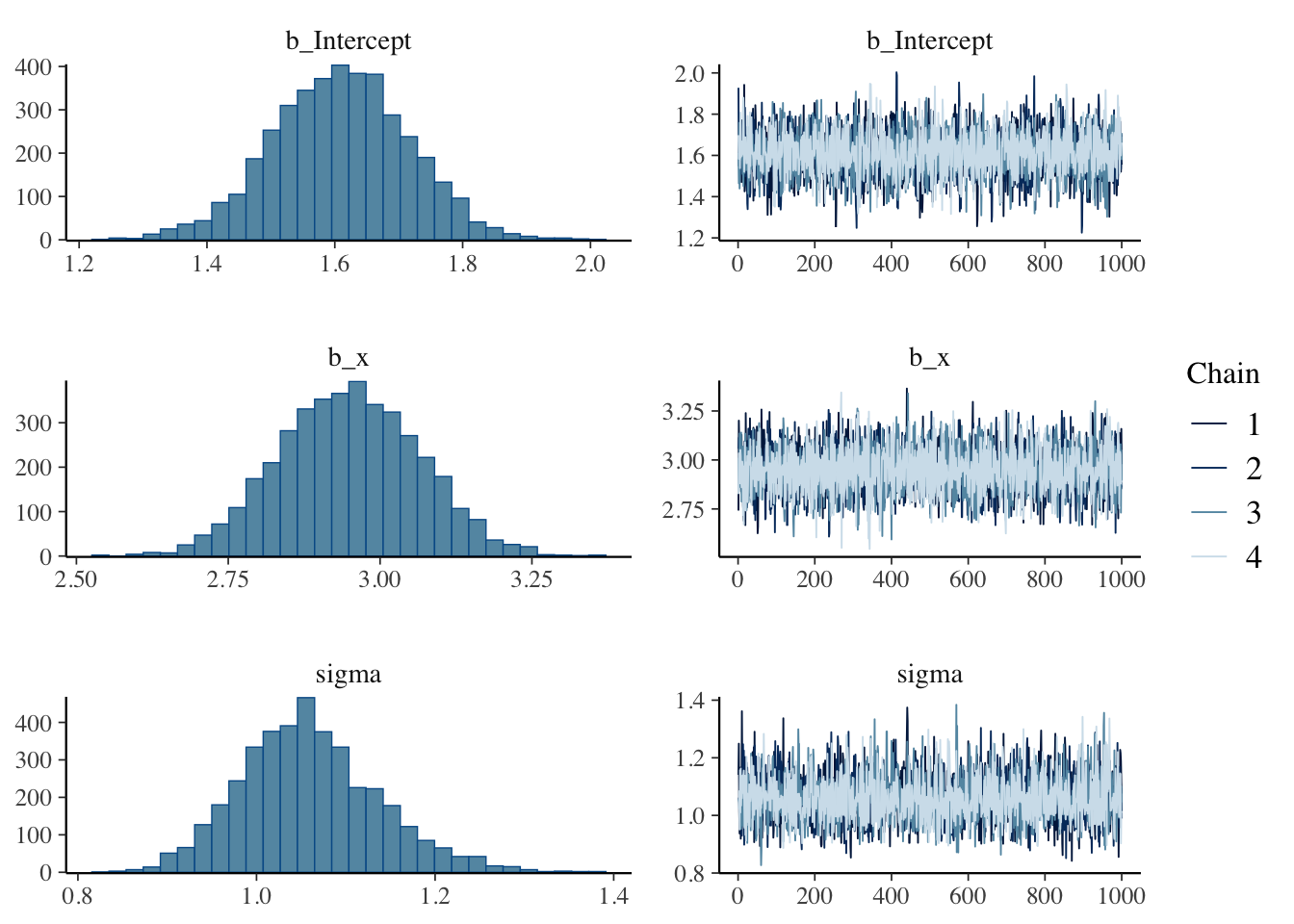
Then build the model with real data.
library(brms)
load("~/Dropbox/github_repos/teaching/POL683_Fall24/advancedRegression/vignettes/dataActive.rda")
dat = dataActive
dat$authoritarianism = scale(dat$authoritarianism)
dat$sdo = scale(dat$sdo)
dat$college = ifelse(dat$educ == "4-year" | dat$educ == "Post-grad", 1, 0)

formula <- bf(sdo ~ authoritarianism + college + authoritarianism:college)

# Specify the priors
priors <- c(
  prior(normal(0, 10), class = "b"),
  prior(normal(0, 10), class = "Intercept"),
  prior(uniform(0, 100), class = "sigma")
)

# Fit the model
fit <- brm(formula, data = dat, prior = priors, chains = 1, iter = 2000, warmup = 1000)
## Running /Library/Frameworks/R.framework/Resources/bin/R CMD SHLIB foo.c
## using C compiler: ‘Apple clang version 16.0.0 (clang-1600.0.26.4)’
## using SDK: ‘’
## clang -arch arm64 -I"/Library/Frameworks/R.framework/Resources/include" -DNDEBUG -I"/Library/Frameworks/R.framework/Versions/4.3-arm64/Resources/library/Rcpp/include/" -I"/Library/Frameworks/R.framework/Versions/4.3-arm64/Resources/library/RcppEigen/include/" -I"/Library/Frameworks/R.framework/Versions/4.3-arm64/Resources/library/RcppEigen/include/unsupported" -I"/Library/Frameworks/R.framework/Versions/4.3-arm64/Resources/library/BH/include" -I"/Library/Frameworks/R.framework/Versions/4.3-arm64/Resources/library/StanHeaders/include/src/" -I"/Library/Frameworks/R.framework/Versions/4.3-arm64/Resources/library/StanHeaders/include/" -I"/Library/Frameworks/R.framework/Versions/4.3-arm64/Resources/library/RcppParallel/include/" -I"/Library/Frameworks/R.framework/Versions/4.3-arm64/Resources/library/rstan/include" -DEIGEN_NO_DEBUG -DBOOST_DISABLE_ASSERTS -DBOOST_PENDING_INTEGER_LOG2_HPP -DSTAN_THREADS -DUSE_STANC3 -DSTRICT_R_HEADERS -DBOOST_PHOENIX_NO_VARIADIC_EXPRESSION -D_HAS_AUTO_PTR_ETC=0 -include '/Library/Frameworks/R.framework/Versions/4.3-arm64/Resources/library/StanHeaders/include/stan/math/prim/fun/Eigen.hpp' -D_REENTRANT -DRCPP_PARALLEL_USE_TBB=1 -I/opt/R/arm64/include -fPIC -falign-functions=64 -Wall -g -O2 -c foo.c -o foo.o
## In file included from <built-in>:1:
## In file included from /Library/Frameworks/R.framework/Versions/4.3-arm64/Resources/library/StanHeaders/include/stan/math/prim/fun/Eigen.hpp:22:
## In file included from /Library/Frameworks/R.framework/Versions/4.3-arm64/Resources/library/RcppEigen/include/Eigen/Dense:1:
## In file included from /Library/Frameworks/R.framework/Versions/4.3-arm64/Resources/library/RcppEigen/include/Eigen/Core:19:
## /Library/Frameworks/R.framework/Versions/4.3-arm64/Resources/library/RcppEigen/include/Eigen/src/Core/util/Macros.h:679:10: fatal error: 'cmath' file not found
## 679 | #include <cmath>
## | ^~~~~~~
## 1 error generated.
## make: *** [foo.o] Error 1
##
## SAMPLING FOR MODEL 'anon_model' NOW (CHAIN 1).
## Chain 1:
## Chain 1: Gradient evaluation took 3.6e-05 seconds
## Chain 1: 1000 transitions using 10 leapfrog steps per transition would take 0.36 seconds.
## Chain 1: Adjust your expectations accordingly!
## Chain 1:
## Chain 1:
## Chain 1: Iteration: 1 / 2000 [ 0%] (Warmup)
## Chain 1: Iteration: 200 / 2000 [ 10%] (Warmup)
## Chain 1: Iteration: 400 / 2000 [ 20%] (Warmup)
## Chain 1: Iteration: 600 / 2000 [ 30%] (Warmup)
## Chain 1: Iteration: 800 / 2000 [ 40%] (Warmup)
## Chain 1: Iteration: 1000 / 2000 [ 50%] (Warmup)
## Chain 1: Iteration: 1001 / 2000 [ 50%] (Sampling)
## Chain 1: Iteration: 1200 / 2000 [ 60%] (Sampling)
## Chain 1: Iteration: 1400 / 2000 [ 70%] (Sampling)
## Chain 1: Iteration: 1600 / 2000 [ 80%] (Sampling)
## Chain 1: Iteration: 1800 / 2000 [ 90%] (Sampling)
## Chain 1: Iteration: 2000 / 2000 [100%] (Sampling)
## Chain 1:
## Chain 1: Elapsed Time: 0.086 seconds (Warm-up)
## Chain 1: 0.081 seconds (Sampling)
## Chain 1: 0.167 seconds (Total)
## Chain 1:## Family: gaussian
## Links: mu = identity; sigma = identity
## Formula: sdo ~ authoritarianism + college + authoritarianism:college
## Data: dat (Number of observations: 3599)
## Draws: 1 chains, each with iter = 2000; warmup = 1000; thin = 1;
## total post-warmup draws = 1000
##
## Regression Coefficients:
## Estimate Est.Error l-95% CI u-95% CI Rhat Bulk_ESS
## Intercept 0.04 0.02 -0.01 0.08 1.00 1121
## authoritarianism 0.26 0.02 0.22 0.30 1.00 827
## college -0.08 0.04 -0.15 -0.01 1.00 1047
## authoritarianism:college 0.11 0.04 0.03 0.18 1.00 928
## Tail_ESS
## Intercept 812
## authoritarianism 837
## college 784
## authoritarianism:college 783
##
## Further Distributional Parameters:
## Estimate Est.Error l-95% CI u-95% CI Rhat Bulk_ESS Tail_ESS
## sigma 0.95 0.01 0.93 0.97 1.00 1020 767
##
## Draws were sampled using sampling(NUTS). For each parameter, Bulk_ESS
## and Tail_ESS are effective sample size measures, and Rhat is the potential
## scale reduction factor on split chains (at convergence, Rhat = 1).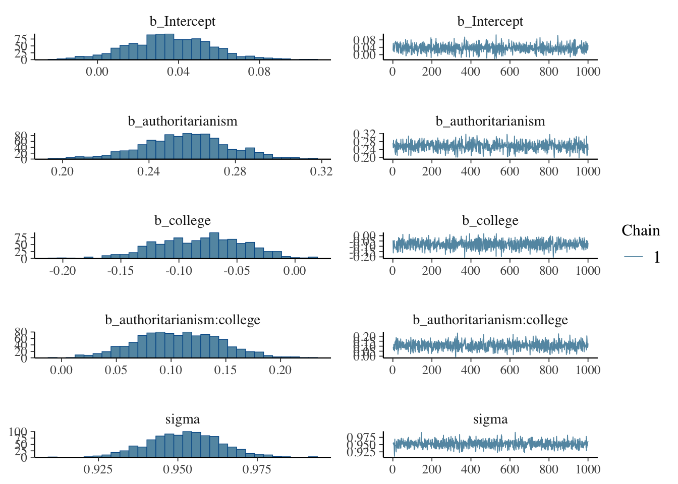
The process of generating posterior predictions is similar to generating predictions from a linear model. We’ll use the \(\texttt{add_epred_draws}\) function to generate predictions from the model. \(\texttt{data_grid}\) comes from the \(\texttt{modelr}\) package; it builds on the \(\texttt{expand.grid}\) fucntion in base R, but it’s a bit more flexible. (Here, it’s identical)
library(tidybayes)
library(dplyr)
library(ggplot2)
library(modelr)
fit <- brm(formula, data = dat, prior = priors, chains = 1, iter = 2000, warmup = 1000)
## Running /Library/Frameworks/R.framework/Resources/bin/R CMD SHLIB foo.c
## using C compiler: ‘Apple clang version 16.0.0 (clang-1600.0.26.4)’
## using SDK: ‘’
## clang -arch arm64 -I"/Library/Frameworks/R.framework/Resources/include" -DNDEBUG -I"/Library/Frameworks/R.framework/Versions/4.3-arm64/Resources/library/Rcpp/include/" -I"/Library/Frameworks/R.framework/Versions/4.3-arm64/Resources/library/RcppEigen/include/" -I"/Library/Frameworks/R.framework/Versions/4.3-arm64/Resources/library/RcppEigen/include/unsupported" -I"/Library/Frameworks/R.framework/Versions/4.3-arm64/Resources/library/BH/include" -I"/Library/Frameworks/R.framework/Versions/4.3-arm64/Resources/library/StanHeaders/include/src/" -I"/Library/Frameworks/R.framework/Versions/4.3-arm64/Resources/library/StanHeaders/include/" -I"/Library/Frameworks/R.framework/Versions/4.3-arm64/Resources/library/RcppParallel/include/" -I"/Library/Frameworks/R.framework/Versions/4.3-arm64/Resources/library/rstan/include" -DEIGEN_NO_DEBUG -DBOOST_DISABLE_ASSERTS -DBOOST_PENDING_INTEGER_LOG2_HPP -DSTAN_THREADS -DUSE_STANC3 -DSTRICT_R_HEADERS -DBOOST_PHOENIX_NO_VARIADIC_EXPRESSION -D_HAS_AUTO_PTR_ETC=0 -include '/Library/Frameworks/R.framework/Versions/4.3-arm64/Resources/library/StanHeaders/include/stan/math/prim/fun/Eigen.hpp' -D_REENTRANT -DRCPP_PARALLEL_USE_TBB=1 -I/opt/R/arm64/include -fPIC -falign-functions=64 -Wall -g -O2 -c foo.c -o foo.o
## In file included from <built-in>:1:
## In file included from /Library/Frameworks/R.framework/Versions/4.3-arm64/Resources/library/StanHeaders/include/stan/math/prim/fun/Eigen.hpp:22:
## In file included from /Library/Frameworks/R.framework/Versions/4.3-arm64/Resources/library/RcppEigen/include/Eigen/Dense:1:
## In file included from /Library/Frameworks/R.framework/Versions/4.3-arm64/Resources/library/RcppEigen/include/Eigen/Core:19:
## /Library/Frameworks/R.framework/Versions/4.3-arm64/Resources/library/RcppEigen/include/Eigen/src/Core/util/Macros.h:679:10: fatal error: 'cmath' file not found
## 679 | #include <cmath>
## | ^~~~~~~
## 1 error generated.
## make: *** [foo.o] Error 1
##
## SAMPLING FOR MODEL 'anon_model' NOW (CHAIN 1).
## Chain 1:
## Chain 1: Gradient evaluation took 3.7e-05 seconds
## Chain 1: 1000 transitions using 10 leapfrog steps per transition would take 0.37 seconds.
## Chain 1: Adjust your expectations accordingly!
## Chain 1:
## Chain 1:
## Chain 1: Iteration: 1 / 2000 [ 0%] (Warmup)
## Chain 1: Iteration: 200 / 2000 [ 10%] (Warmup)
## Chain 1: Iteration: 400 / 2000 [ 20%] (Warmup)
## Chain 1: Iteration: 600 / 2000 [ 30%] (Warmup)
## Chain 1: Iteration: 800 / 2000 [ 40%] (Warmup)
## Chain 1: Iteration: 1000 / 2000 [ 50%] (Warmup)
## Chain 1: Iteration: 1001 / 2000 [ 50%] (Sampling)
## Chain 1: Iteration: 1200 / 2000 [ 60%] (Sampling)
## Chain 1: Iteration: 1400 / 2000 [ 70%] (Sampling)
## Chain 1: Iteration: 1600 / 2000 [ 80%] (Sampling)
## Chain 1: Iteration: 1800 / 2000 [ 90%] (Sampling)
## Chain 1: Iteration: 2000 / 2000 [100%] (Sampling)
## Chain 1:
## Chain 1: Elapsed Time: 0.088 seconds (Warm-up)
## Chain 1: 0.088 seconds (Sampling)
## Chain 1: 0.176 seconds (Total)
## Chain 1:dat %>% data_grid( authoritarianism = seq_range(authoritarianism, n = 30),
college = c(0, 1)) %>%
add_epred_draws(fit) %>%
group_by(authoritarianism, college) %>%
mutate(college = ifelse(college == 1, "College", "Less than College")) %>%
summarize(
.value = mean(.epred),
.lower = quantile(.epred, 0.025),
.upper = quantile(.epred, 0.975)
) %>%
ggplot(aes(x = authoritarianism, y = .value, color = factor(college))) +
geom_line() +
geom_ribbon(aes(ymin = .lower, ymax = .upper), alpha = 0.3) +
facet_wrap(~college) +
labs(
x = "Authoritarianism",
y = "Social Dominance Orientation",
color = "Education",
title = "Predicted Social Dominance Orientation \nby Authoritarianism and Education"
) +
theme_minimal()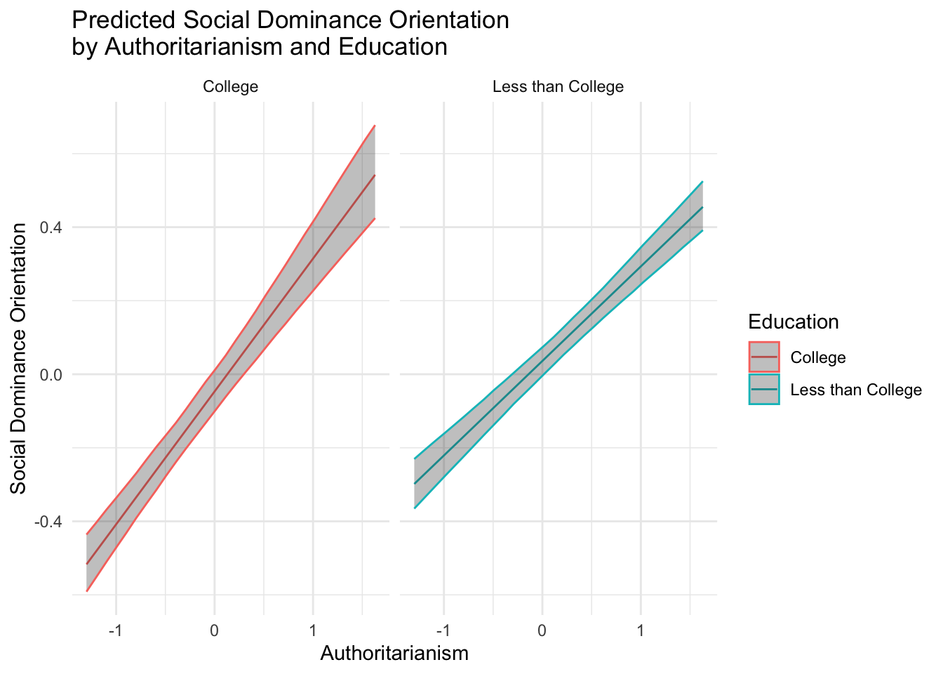
5.5 Building a Model
Simulation can be a powerful tool, beyond just generating predictions – posterior or point. It allows us to test underlying assumptions in our models.
In Chapter 2 we discussed the Directed Acyclic Graph – DAG - and how this is a useful tool to represent theoretical relationships and build both statistical and causal models. If we focus solely on association as opposed to causation, it is entirely conceivable that you’ll document some strange relationships, like a positive association between the number of waffle houses in a state, and that state’s divorce rate (McElreath 2022), or the positive relationship between per capita ice-cream consumption and death rates among minors. If we solely focus on the statistical, ignoring the scientific these kind of counter-intuitive, downright strange relationships abound.
5.6 Steps to Building a Model
Build a scientific model. This is the theoretical model that you believe underlies the data. This is often represented in a DAG.
Build a statistical model. How might we use a statistical model to create estimands – parameters that we’ll estimate with our data?
Estimation, Simulation and Prediction. Here we’ll join the statistical and scientific model, using the data to test associations and causal processes.
5.7 The DAG
5.7.1 Conservatism and Age
The DAG depicts a theoretical relationship between variables. Let’s start simple, the relationship between age and conservatism. We’re probably all familiar with this problematic “quote.”
“If you’re not a liberal when you’re 25, you have no heart. If you’re not a conservative by the time you’re 35, you have no brain.”
This the infamous quote, falsely attribute to Winston Churchill.There’s no evidence he actually said this, but in any case, folk wisdom seems to similar point to this.
As the story goes, when one ages in a post industrial market economy, they develop financial (e.g., home and car ownership) and social capital (e.g., promotions, power). As an ideology, conservatism tends to correlate with lower taxes, a smaller size (and scope) of federal government, and a preference to free market to government solutions. Throughout the lifespan, one accumulates more wealth, subsequently developing a personal interest in maintaining such wealth.
Continuing on, when one reaches retirement age – the story goes – a senior has less “skin in the game,” as their children are grown and they are no longer working. These individuals, on average, are even less likely to favor liberal social welfare programs. And of course we have observational/anecdotal evidence supporting such a narrative. Just look to retirement states – like Arizona and Florida – where social welfare programs are meager.
Though this is the folk narrative, there is relatively little empirical evidence to support this notion. Peterson, Smith and Hibbing (2020) show no relationship between age and conservatism, instead document remarkable stability in political attitudes over the life course. Likewise, Alford, Funk, and Hibbing (2005) show that political attitudes are partially heritable, and that genetic factors explain a significant portion of the variance in political ideology. In psychology, John Jost and colleagues (Jost et al 2004) show that conservatism is firmly rooted in stable personality traits – like authoritarianism and social dominance orientation – and epistemic goals (e.g., need for cognitive closure). These empirical investigations develop a very different narrative: Ideology is a relatively stable expression of psychological and even biological predispositions.
Let’s use this to develop different DAGs, simulate data, generate causal estimands, and test the relationship between age and conservatism. We’ll start with a simple model, moving to a more complex model, all the while considering the role of age in causing political conservatism.
Here’s the simple model:
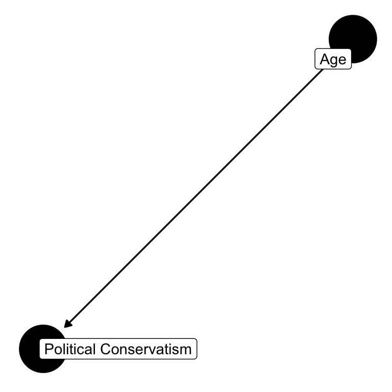
Let’s also not hide our interests in cause-and-effect in imprecise language, like “association,” “correlation,” and “relationships.” While we’re interested in these things, assume our core interest is in causation. Does age causally impact conservatism? I’ll say more about causation in the next chapter. For our purposes now, it’s sufficient to note that we can often sort out how to create causal estimands by simply drawing a graphical depiction of how variables relate to one another, the DAG.
5.8 The Confound
5.8.1 The Fork
Here’s the simple model:
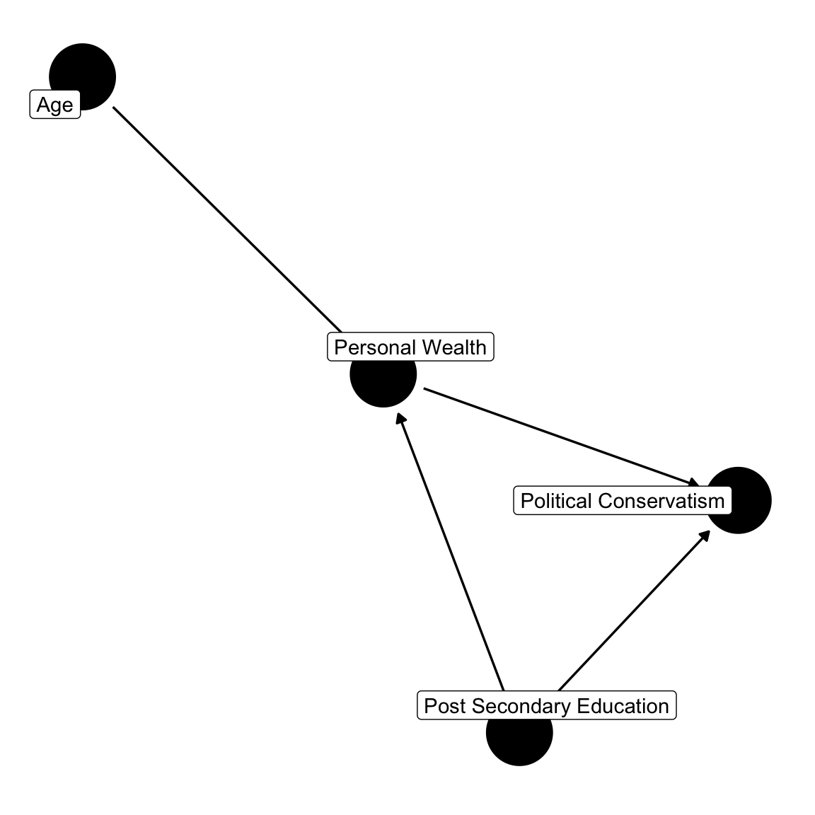
This seems to be a plausible graph – age influences the accumulation of personal wealth, personal wealth perhaps leads to conservatism, with the goal of maximizing one’s wealth. Again, fiscal conservatism advocates a smaller federal government, lower taxes, and less regulation. However, post-secondary education also relates to personal wealth – as a college degree generally translates to higher paying jobs. Post-secondary education is also related to political conservatism. But in the United States, it’s typically found that college and graduate degrees translate to political liberalism. Let’s ignore age for the time being, focusing on post-secondary education, the fork.
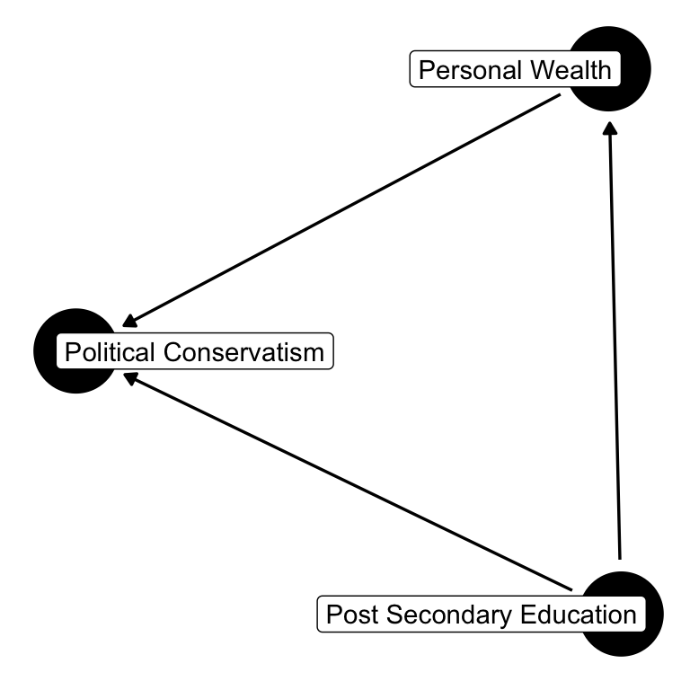
Post-secondary education is a “confounding” variable. The relationship between personal wealth and political conservatism might be spurious if one were to ignore post-secondary education. If education is a confound, failing to condition on education, a common cause of both personal wealth and political conservatism, means that if we ignore education, the independence will no longer hold.
Let’s simulate a world in which education is a confound. We’ll simulate a population in which 30% has a college or post-graduate degree. We’ll then predict personal wealth and political conservatism. We’ll then compare the relationship between wealth and conservatism, conditioning on education, and not conditioning on education.
##
## Call:
## lm(formula = political_conservatism ~ wealth)
##
## Residuals:
##     Min      1Q  Median      3Q     Max
## -3.5958 -0.6836  0.0392  0.7159  3.4477
##
## Coefficients:
##             Estimate Std. Error t value Pr(>|t|)
## (Intercept)  1.63460    0.07093  23.045   <2e-16 ***
## wealth       0.12517    0.05298   2.363   0.0183 *
## ---
## Signif. codes:  0 '***' 0.001 '**' 0.01 '*' 0.05 '.' 0.1 ' ' 1
##
## Residual standard error: 1.036 on 998 degrees of freedom
## Multiple R-squared:  0.005563,   Adjusted R-squared:  0.004566
## F-statistic: 5.583 on 1 and 998 DF,  p-value: 0.01833
##
## Call:
## lm(formula = political_conservatism ~ wealth + education)
##
## Residuals:
## Min 1Q Median 3Q Max
## -3.6410 -0.6947 0.0629 0.7229 3.3963
##
## Coefficients:
## Estimate Std. Error t value Pr(>|t|)
## (Intercept) 1.48630 0.07249 20.503 < 2e-16 ***
## wealth 0.39300 0.06447 6.096 1.55e-09 ***
## education -0.62417 0.08958 -6.968 5.85e-12 ***
## ---
## Signif. codes: 0 '***' 0.001 '**' 0.01 '*' 0.05 '.' 0.1 ' ' 1
##
## Residual standard error: 1.012 on 997 degrees of freedom
## Multiple R-squared: 0.05174, Adjusted R-squared: 0.04983
## F-statistic: 27.2 on 2 and 997 DF, p-value: 3.156e-12## wealth
## 0.2678279The difference between the wealth coefficient in the two models is fairly substantial. It’s attenuated in the equation without education – why? – and considerably larger (and signed in the conservative direction) in the model that includes education.
We can simulate this experiment a bunch of times, varying the sample size, and number of trials.
In these simulations, notice that the difference between these coefficients hovers around 0.2, with a range from 0.15 to 0.33 or so. In this fictitious example, wealth is related to political conservatism. But, when we condition on education, the relationship between wealth and conservatism changes. According to our scientific model, education predicts both wealth and conservatism. It is a confound. It should not be ignored.
Though our interest is in age and conservatism let’s say we want to generate a causal estimate of wealth. How does wealth causally impact political conservatism?
In the next chapter, we’ll consider causation further, by building upon the DAGs in this chapter, while also elaborating on a common language used to express causal relationships.